5.1 Infinity, limits, and power functions
Activity 5.1.2
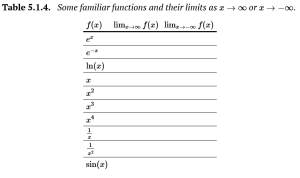
Complete the Table 5.1.4 by entering “[latex]\infty[/latex],” “[latex]-\infty[/latex],” “0,” or “no limit” to identify how the function behaves as either [latex]x[/latex] increases or decreases without bound. As much as possible, work to decide the behavior without using a graphing utility.
Show Solution
| [latex]f(x)[/latex] | [latex]\lim_{x \to -\infty} f(x)[/latex] | [latex]\lim_{x \to \infty} f(x)[/latex] |
| [latex]e^x[/latex] | [latex]\infty[/latex] | [latex]0[/latex] |
| [latex]e^{-x}[/latex] | [latex]0[/latex] | [latex]\infty[/latex] |
| [latex]\ln (x)[/latex] | [latex]\infty[/latex] | does not exist |
| [latex]x[/latex] | [latex]\infty[/latex] | [latex]-\infty[/latex] |
| [latex]x^2[/latex] | [latex]\infty[/latex] | [latex]\infty[/latex] |
| [latex]x^3[/latex] | [latex]-\infty[/latex] | [latex]\infty[/latex] |
| [latex]x^4[/latex] | [latex]\infty[/latex] | [latex]\infty[/latex] |
| [latex]\frac{1}{x}[/latex] | [latex]0[/latex] | [latex]0[/latex] |
| [latex]\frac{1}{x^2}[/latex] | [latex]0[/latex] | [latex]0[/latex] |
| [latex]\sin (x)[/latex] | no limit | no limit |
Activity 5.1.3
Point your browser to the Desmos worksheet at http://gvsu.edu/s/0zu. In what follows, we explore the behavior of power functions of the form [latex]y=x^n[/latex] where [latex]n\geq 1[/latex].
a. Press the “play” button next to the slider labeled “[latex]n[/latex]". Watch at least two loops of the animation and then discuss the trends that you observe. Write a careful sentence each for at least two different trends.
b. Click the icons next to each of the following 8 functions so that you can see all of [latex]y=x, y=x^2, ..., y=x^8[/latex] graphed at once. On the interval [latex]0[/latex] < [latex]x[/latex] < [latex]1[/latex], how do the graphs of [latex]x^a[/latex] and [latex]x^b[/latex] compare if [latex]a[/latex] < [latex]b[/latex]?
c. Uncheck the icons on each of the 8 functions to hide their graphs. Click the settings icon to change the domain settings for the axes, and change them to [latex]-10 \leq x \leq 10[/latex] and [latex]-10,000 \leq y \leq 10,000[/latex]. Play the animation through twice and then discuss the trends that you observe. Write a careful sentence each for at least two different trends.
d. Click the icons next to each of the following 8 functions so that you can see all of [latex]y=x, y=x^2, …, y=x^8[/latex] graphed at once. On the interval [latex]x>1[/latex], how do the graphs of [latex]x^a[/latex] and [latex]x^b[/latex] compare if [latex]a < b[/latex]?
Show Solution
a. When the power is odd, the graph is increasing, but when the power is even, the graph decreases first, then increases. Also, the graphs are always present in the first quadrant, but alternate between the second and the third quadrants, depending on odd or even power.
b. On [latex]0[/latex]< [latex]x[/latex] < [latex]1[/latex], all graphs are increasing. When specifically looking at graphs of [latex]x^a[/latex] and [latex]x^b[/latex] compare if [latex]a < b[/latex], we see that [latex]x^a > x^b[/latex].
c. The larger the power, the quicker the function increase as [latex]x[/latex] gets larger. The portion of the graph when [latex]x[/latex] < [latex]0[/latex] alternates between the second and third quadrants depending on if the power is odd or even.
d. When [latex]x > 1[/latex] and [latex]a < b[/latex], [latex]x^a < x^b[/latex].
Activity 5.1.4
Point your browser to the Desmos worksheet at http://gvsu.edu/s/0zv. In what follows, we explore the behavior of power functions [latex]y=x^n[/latex] where [latex]n \leq −1[/latex].
a. Press the “play” button next to the slider labeled “[latex]n[/latex].” Watch two loops of the animation and then discuss the trends that you observe. Write a careful sentence each for at least two different trends.
b. Click the icons next to each of the following 8 functions so that you can see all of [latex]y=x^{-1}, y=x^{-2}, …, y=x^{-8}[/latex] graphed at once. On the interval [latex]1[/latex] < [latex]x[/latex], how do the functions [latex]x^a[/latex] and [latex]x^b[/latex] compare if [latex]a[/latex] < [latex]b[/latex]? (Be careful with negative numbers here: e.g., [latex]-3[/latex] < [latex]-2[/latex].)
c. How do your answers change on the interval [latex]0[/latex] < [latex]x[/latex] < [latex]1[/latex]?
d. Uncheck the icons on each of the 8 functions to hide their graphs. Click the settings icon to change the domain settings for the axes, and change them to [latex]-10\leq x \leq 10[/latex] and [latex]-10,000 \leq y \leq 10,000[/latex]. Play the animation through twice and then discuss the trends that you observe. Write a careful sentence each for at least two different trends.
e. Explain why [latex]\lim_{x \to \infty} \frac{1}{x^n}=0[/latex] for any choice of [latex]n=1,2,….[/latex]
Show Solution
a. As [latex]n[/latex] increases, the functions get closer to the [latex]x[/latex]-axis faster. For all [latex]n[/latex], a portion of the graph is in the first quadrant, but when [latex]n[/latex] is odd, the second portion is in the third quadrant, while when [latex]n[/latex] is even, the second portion is in the second quadrant.
b. When [latex]a < b[/latex], [latex]x^a < x^b[/latex] for [latex]x > 1[/latex].
c. [latex]x^a > x^b[/latex]
d. As [latex]n[/latex] increases, the graphs move further away from the [latex]y[/latex]-axis. For all [latex]n[/latex], the graphs appear in the first quadrant, but the second piece of each graph will either be in the second or third quadrants, depending on if [latex]n[/latex] is even or odd.
e. In all cases, a very large value for [latex]x[/latex] is raised to a positive power makes for an even larger value. 1 divided by an ever increasing large number approaches 0.
5.1 Exercise 5
Consider the familiar graph of [latex]f(x)=\frac{1}{x}[/latex], which has a vertical asymptote at [latex]x=0[/latex] and a horizontal asymptote at [latex]y=0[/latex], as pictured in Figure 5.1.8. In addition, consider the similarly-shaped function [latex]g[/latex] shown in Figure 5.1.9, which has vertical asymptote [latex]x=-1[/latex] and horizontal asymptote [latex]y=-2[/latex].
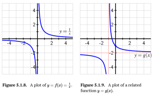
a. How can we view [latex]g[/latex] as a transformation of [latex]f[/latex]? Explain, and state how [latex]g[/latex] can be expressed algebraically in terms of [latex]f[/latex].
b. Find a formula for [latex]g[/latex] as a function of [latex]x[/latex]. What is the domain of [latex]g[/latex]?
c. Explain algebraically (using the form of [latex]g[/latex] from (b)) why [latex]\lim_{x \to \infty} g(x)=-2[/latex] and [latex]\lim_{x \to -1} g(x)=\infty[/latex].
d. What if a function [latex]h[/latex] (again of a similar shape as [latex]f[/latex]) has vertical asymptote [latex]x=5[/latex] and horizontal asymptote [latex]y=10[/latex]. What is a possible formula for [latex]h(x)[/latex]?
e. Suppose that [latex]r(x)=\frac{1}{x+35}-27[/latex]. Without using a graphing utility, how do you expect the graph of [latex]r[/latex] to appear? Does it have a horizontal asymptote? A vertical asymptote? What is its domain?
Show Solution
a. [latex]f[/latex] has been shifted left [latex]1[/latex] and down [latex]2[/latex], [latex]g(x)=f(x+1)-2[/latex].
b. [latex]g(x)=\frac{1}{x+1}-2[/latex]. Domain: [latex](-\infty,-1)\bigcup(-1,\infty)[/latex]
c. For [latex]\lim_{x \to \infty} g(x)=-2[/latex], in the [latex]g(x)[/latex] function, the fraction [latex]\frac{1}{x+1}[/latex] approaches [latex]0[/latex] as [latex]x[/latex] increases. Then [latex]0-2[/latex] is [latex]-2[/latex].
For [latex]\lim_{x \to -1} g(x)=\infty[/latex], in the [latex]g(x)[/latex] function, the fraction [latex]\frac{1}{x+1}[/latex] will approach [latex]\infty[/latex]. So [latex]\infty-2[/latex] will still be [latex]\infty[/latex].
d. [latex]h(x)=\frac{1}{x-5}+10[/latex]
e. This graph will have the same shape as [latex]\frac{1}{x}[/latex], but have a horizontal asymptote [latex]y=-27[/latex] and a vertical asymptote [latex]x=-35[/latex]. Domain: [latex](-\infty, -35)\bigcup (-35,\infty)[/latex].
