5 Week 4 Normal Distributions Reading

An Introduction

The normal distribution, a continuous distribution, is the most important of all the distributions. It is widely used and even more widely abused. Its graph is bell-shaped, i.e. symmetric. You encounter the bell curve in almost all disciplines. Some of these include psychology, business, economics, the physical sciences, nursing, and, of course, mathematics. Some of your instructors may use the normal distribution to help determine your course grade. Most IQ scores are normally distributed. Often real estate prices fit a normal distribution, as do female shoe sizes, heights of people, blood pressures, and newborn baby weights.

In this section, you will study the normal distribution, the standard normal distribution, and applications associated with them.

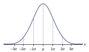
In a normal distribution, the mean in centrally located, and standard deviation is used as the best measure of variability.  In Statistics, the Greek letter mu ( ) is used to represent population mean.  , sigma, represents the population standard deviation.  Both of these symbols are seen in the graph above.  Notice the mean as the center with increments marked in terms of number of standard deviations to the left and right, as part of the normal shape.

Calculating Z-Scores

Z-scores are standardized values that tell you how many standard deviations a particular data value is from the mean.  Z-scores are particularly useful when you want to compare data from two or more distributions.

To calculate a Z-score, you need the mean and standard deviation of the distribution, as well as the observed value (X).

This formula can also be used when the Z-score is known, and you want to calculate the observed (raw) score (X), that it corresponds to.

Example: Newborn baby weights, in grams, follow a normal distribution. For the purpose of this example, we will look at babies born at 40 weeks.  Babies of European descent have an average birth weight of 3687.6 g with a standard deviation of 419.6. Babies of Chinese descent have an average birth weight of 3600.4 g with a standard deviation of 343.5.

Let’s say that a baby was born at 4000 g. Is this weight more unusual if the baby is of European descent or Chinese descent?

First, let’s calculate the Z-scores for each of the backgrounds.

European:  

This means that if of European descent, a baby weight of 4000 g is 0.74 standard deviations above the mean of 3687.6 g.

Chinese:

This means that if of Chinese descent, a baby weight of 4000 g is 1.16 standard deviations above the mean of 3600.4 g

Looking at the Z-scores, 1.16 is a larger value than 0.74 meaning that 4000 g is a more unusual weight with respect to the Chinese distribution than the European distribution.  The further a Z-score is from 0, the more unusual the observation.

For another look at Z-scores,  Khan Academy on Calculating Z scores [7:47].

Standard Normal curves are curves where the mean is 0, and the standard deviation  is 1.  The standard normal curve is the distribution of Z-scores.

The Empirical Rule (aka 68-95-99.7 rule)

In a normal distribution with mean µ and standard deviation σ, the Empirical Rule states the following:

• About 68% of the data lie between –1σ and +1σ of the mean µ (within one standard deviation of the mean).
• About 95% of the data lie between –2σ and +2σ of the mean µ (within two standard deviations of the mean).
• About 99.7% of the data lie between –3σ and +3σ of the mean µ (within three standard deviations of the mean).

Notice that almost all the data lie within three standard deviations of the mean.

In Statistics, the further data is from the mean, the more unusual that data is considered to be.  Generally speaking, data that falls more than 2 standard deviations from the mean (outside the middle 95%) is considered to be unusual enough to question whether the assumed mean value is actually correct.  This will be studied in much further depth later in the semester when we learn about formal hypothesis testing.

With data that is approximately normal, you can use your knowledge of the curve’s symmetry and percentages under the curve to estimate the percentile rank of particular data values.  Recall from earlier in the semester, we defined percentile ranks as the percentage of subject at a particular value/interval or below.

Example: A certain IQ test has a mean of 100, and a standard deviation of 8.  Here is a the label curve with three standard deviations in both directions.

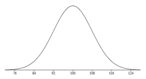Perhaps you want to know what percentage of test takers score a 100 or less.  Since 100 is the mean, it is the middle of the curve, where 50% of the data lies below.   In other words, 50% of the test takers earn a 100 or less.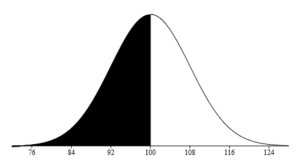If you were interested in the percentile rank of someone with a score of 92, you’d look below the mean, and automatically know that this percentile rank should be less than 50%.  Since 92 is exactly 1 standard deviation below the mean, that would make this percentile rank 16%.  Looking at the graph below, you add up the percentages that fall below -1 on the curve.  16% of the test takers had a score of 92 or less.

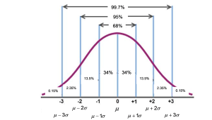
On the other hand, what if you wanted to know the percentile rank of someone with an IQ score of 116?  A score of 116 is two standard deviation above the mean, so you know that the percentile rank should be greater than 50%. Looking at the same graph below, find the vertical line at +2 standard deviation above the mean, then add up the percentages that fall to the left.  We end up with 97.5% which tells us that 97.5% of the test takers have an IQ score of 116 or less.

To view more about the estimation of percentile ranks using the Empirical Rule: Khan Academy on Estimating Percentile Rank using 69%, 95%, 99.7% Rule [7:41].

Student Course Learning Objectives

2.  Describe data both graphically and numerically

h.  Use 68%, 95%, 99.7% estimates

i.  Calculate z-scores

j.  Calculate proportion of values under the curve, including percentile ranks

6. Communicate in writing the results of statistical analyses of data

Attributions

Adapted from “Week 4 Normal Distributions Reading” by Sherri Spriggs and Sandi Dang is licensed under CC BY-NC-SA 4.0.